Plot that Euler Method Graph
Euler Method is widely used in various fields such as physics, engineering, and finance for solving differential equations that describe dynamic systems. It is particularly useful for initial exploratory analysis and for problems where a high degree of precision is not required.
Geometrically, Euler's method approximates the curve of the solution by a series of tangent line segments. At each step, the slope of the tangent is given by the differential equation 𝑓(𝑥,𝑦)f(x,y).
I have commented the Rust code for you to follow through.
The Rust code
// A program to make a graph of the Euler Method.
// Inputs of 0.1 for x, y and steplength and
// 10 for number of steps works well.
// by Rich from https://maths.earth/

use std::f64::consts::E;
use std::io::{self, Write};
use plotters::prelude::*;
use minifb::{Key, Window, WindowOptions};

// Function definition for the differential equation y' = 2y.
fn differential_equation(_x: f64, y: f64) -> f64 {
    2.0 * y
}

fn main() {
    // String representation of the differential equation for display purposes.
    let equation_string = "y' = 2y";
    println!("Solving the equation {} using Euler's method and Midpoint method.", equation_string);

    // Prompt user for initial values of x and y, step length, and number of steps.
    print!("Initial values, x = ");
    io::stdout().flush().unwrap();
    let mut x_value: f64 = read_input();

    print!("                y = ");
    io::stdout().flush().unwrap();
    let mut approx_y_value: f64 = read_input();

    print!("      step length = ");
    io::stdout().flush().unwrap();
    let step_length: f64 = read_input();

    print!("  number of steps = ");
    io::stdout().flush().unwrap();
    let num_steps: i32 = read_input() as i32;

    println!();

    // Calculate the constant of integration based on the initial values.
    let constant_of_integration = approx_y_value / E.powf(2.0 * x_value);

    // Print table header for x, approximate y, and exact y values.
    println!("{:>6} {:>16} {:>16} {:>16}", "x", "approx y (Euler)", "approx y (Midpoint)", "exact y");
    println!("{:>6} {:>16} {:>16} {:>16}", "-", "----------------", "-----------------", "-------");

    // Vectors to store x values, Euler's method y values, Midpoint method y values, and exact y values.
    let mut x_values = vec![];
    let mut approx_y_values_euler = vec![];
    let mut approx_y_values_midpoint = vec![];
    let mut exact_y_values = vec![];

    // Initialize the Midpoint method variable.
    let mut approx_y_value_midpoint = approx_y_value;

    // Iterate through the number of steps to calculate values using both methods.
    for _ in 1..=num_steps {
        // Euler's method update for approx_y_value.
        approx_y_value = approx_y_value + step_length * differential_equation(x_value, approx_y_value);

        // Midpoint method update for approx_y_value_midpoint.
        let mid_x = x_value + step_length / 2.0;
        let mid_y = approx_y_value_midpoint + (step_length / 2.0) * differential_equation(x_value, approx_y_value_midpoint);
        approx_y_value_midpoint = approx_y_value_midpoint + step_length * differential_equation(mid_x, mid_y);

        // Update x_value by adding the step length.
        x_value = x_value + step_length;

        // Append current x_value, approx_y_value (Euler), approx_y_value_midpoint, and exact_y_value to their respective vectors.
        x_values.push(x_value);
        approx_y_values_euler.push(approx_y_value);
        approx_y_values_midpoint.push(approx_y_value_midpoint);
        exact_y_values.push(constant_of_integration * E.powf(2.0 * x_value));

        // Print current step values.
        println!("{:>6.2} {:>16.10} {:>16.10} {:>16.10}", x_value, approx_y_value, approx_y_value_midpoint, constant_of_integration * E.powf(2.0 * x_value));
    }

    // Plot the results of the approximations and the exact solution.
    plot_results(&x_values, &approx_y_values_euler, &approx_y_values_midpoint, &exact_y_values).unwrap();

    // Display the graph in a window.
    display_graph_in_window().unwrap();
}

// Function to read and parse user input.
fn read_input() -> f64 {
    let mut input = String::new();
    io::stdin().read_line(&mut input).expect("Failed to read line");
    input.trim().parse().ok().expect("Invalid input")
}

// Function to plot the results using the plotters crate.
fn plot_results(x_values: &Vec<f64>, approx_y_values_euler: &Vec<f64>, approx_y_values_midpoint: &Vec<f64>, exact_y_values: &Vec<f64>) -> Result<(), Box<dyn std::error::Error>> {
    let root_area = BitMapBackend::new("euler_method.png", (640, 480)).into_drawing_area();
    root_area.fill(&WHITE)?;

    let mut chart = ChartBuilder::on(&root_area)
        .caption("Euler's Method Approximations", ("sans-serif", 50).into_font())
        .margin(10)
        .x_label_area_size(30)
        .y_label_area_size(30)
        .build_cartesian_2d(
            *x_values.first().unwrap()..*x_values.last().unwrap(),
            *approx_y_values_euler.iter().min_by(|a, b| a.partial_cmp(b).unwrap()).unwrap()
                ..*exact_y_values.iter().max_by(|a, b| a.partial_cmp(b).unwrap()).unwrap(),
        )?;

    chart.configure_mesh().draw()?;

    // Plot the approximate y values using Euler's method.
    chart.draw_series(LineSeries::new(
        x_values.iter().zip(approx_y_values_euler.iter()).map(|(&x, &y)| (x, y)),
        &BLUE,
    ))?
    .label("Approx y (Euler)")
    .legend(|(x, y)| PathElement::new(vec![(x, y), (x + 20, y)], &BLUE));

    // Plot the approximate y values using the Midpoint method.
    chart.draw_series(LineSeries::new(
        x_values.iter().zip(approx_y_values_midpoint.iter()).map(|(&x, &y)| (x, y)),
        &GREEN,
    ))?
    .label("Approx y (Midpoint)")
    .legend(|(x, y)| PathElement::new(vec![(x, y), (x + 20, y)], &GREEN));

    // Plot the exact y values.
    chart.draw_series(LineSeries::new(
        x_values.iter().zip(exact_y_values.iter()).map(|(&x, &y)| (x, y)),
        &RED,
    ))?
    .label("Exact y")
    .legend(|(x, y)| PathElement::new(vec![(x, y), (x + 20, y)], &RED));

    chart.configure_series_labels()
        .background_style(&WHITE.mix(0.8))
        .border_style(&BLACK)
        .draw()?;

    root_area.present()?;
    println!("Result has been saved to euler_method.png");

    Ok(())
}

// Function to display the graph in a window using the minifb crate.
fn display_graph_in_window() -> Result<(), Box<dyn std::error::Error>> {
    let img = image::open("euler_method.png")?.to_rgba8();
    let (width, height) = img.dimensions();
    let buffer: Vec<u32> = img
        .pixels()
        .map(|p| {
            let [r, g, b, _] = p.0;
            ((r as u32) << 16) | ((g as u32) << 8) | (b as u32)
        })
        .collect();

    let mut window = Window::new(
        "Euler's Method Graph - ESC to exit",
        width as usize,
        height as usize,
        WindowOptions::default(),
    )?;

    // Keep the window open until the user presses the Escape key.
    while window.is_open() && !window.is_key_down(Key::Escape) {
        window.update_with_buffer(&buffer, width as usize, height as usize)?;
    }

    Ok(())
}
Cargo.toml
[package]
name = "euler"
version = "0.1.0"
edition = "2021"

[dependencies]
plotters = "0.3.6"
minifb = "0.27.0"
image = "0.25.1"
The image produced:
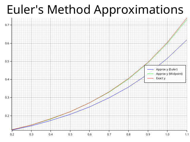
Mission Accomplished
And there we have it, we have a graph on the screen and a graph in a file of the Euler Method compared to the Midpoint Method.